Introduction of the Cloud Resolving Storm Simulator (CReSS)
|
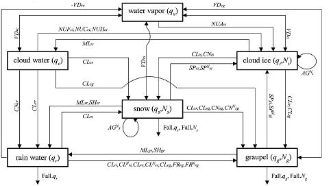
The formulation of CReSS is based on the non-hydrostatic and compressible equation using terrain-following coordinates. Prognostic variables are 3-dimensional velocity components, perturbations of pressure and potential temperature, water vapor mixing ratio, sub-grid scale turbulent kinetic energy (TKE), and cloud physical variables. A finite difference method is used for the spatial discretization. The horizontal domain is rectangular, and variables are set on a staggered grid: the Arakawa-C grid in the horizontal and the Lorenz grid in the vertical. For time integration, the mode-splitting technique (Klemp and Wilhelmson 1978) is used. Terms related to sound waves of the basic equation are integrated with a small time step, and other terms with a large time step. Cloud physical processes are formulated by a bulk method of cold rain, which is based on Lin et al. (1983), Cotton et al. (1986), Murakami (1990), Ikawa and Saito (1991), and Murakami et al. (1994). The bulk parameterization of cold rain considers water vapor, rain, cloud, ice, snow, and graupel. The microphysical processes implemented in the model are described in Fig.1. |
|
| Figure 1: Diagram describing water substances and cloud microphysical processes in the bulk scheme of CReSS. (Tsuboki and Sakakibara, 2002) |
|
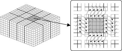
Parameterizations of the sub-grid scale eddy motions in CReSS are one-order closure of Smagorinsky (1963) or the 1.5-order closure of turbulent kinetic energy (TKE). In the latter parameterization, the prognostic equation of TKE is used. All numerical experiments in this textbook use three-dimensional 1.5-order closure scheme. The surface process of CReSS is formulated by a bulk method, whose bulk coefficients are taken from Louis et al. (1981). Several types of initial and boundary conditions are available. For a numerical experiment, a horizontally uniform initial field provided by a sounding profile will be used with an initial disturbance of a thermal bubble or random temperature perturbation. The boundary conditions are one of the following types; rigid wall, periodic, zero normal-gradient, and wave-radiation types. CReSS can be nested within a coarse-grid model for a prediction experiment. In such an experiment, the initial field is provided by interpolating grid-point values and the boundary condition is provided by the coarse-grid model. For a computation within a large domain, conformal map projections are available, which include the Lambert conformal projection, the polar stereographic projection, and the Mercator projection. For parallel computing of a large computation, CReSS provides two-dimensional domain decomposition in the horizontal direction (Fig.2). Parallel processing is performed using the Massage Passing Interface (MPI). Communications between individual processing elements (PEs) are performed by exchanging data of the two outermost grids. The OpenMP is also available. |
|
| Figure 2: Schematic representation of two-dimensional domain decomposition and the communication strategy for parallel computations using MPI. |
|
References
|